10. numpyの基本と応用

numpyは、科学技術計算を容易にかつ高速に実現するために開発されたライブ ラリです。これまでに学んだ知識を使ってリストや多次元配列にデータをため て、for文等で配列のデータにアクセスできますが、データが巨大になると圧 倒的に遅くなります。numpyを使うことで、多次元配列の処理を簡潔に書けて 高速に処理できるようになります。またnumpyは、数学関数や乱数発生、線形 代数、統計処理、データの入出力等、科学技術計算で基本となる非常に豊富な 機能を提供しています。

https://docs.scipy.org/doc/numpy-1.13.0/reference/

今回の学習目標は以下のとおりです。

• numpyでの配列操作(indexing, broadcasting)を理解する。

• numpyで使える代表的な関数を理解する。

• numpyで線形代数計算、統計処理を行う理解する。

なお慣習にしたがって、numpytは別名npとしてimportします。

example-01

import numpy as np   # npとしてnumpyをimport (慣例)

多次元配列とデータ型

リスト変数をnp.array()を使って配列(array)オブジェクトを生成します。多 次元リストのようにサイズの異なる要素になることはできません。np.array() で生成したインスタンスは、要素数、形(行と列数)、型等は、クラス変数 (size, shpae, dtype等)として保持しています。

https://docs.scipy.org/doc/numpy-1.13.0/reference/generated/numpy.ndarray.html

example-02

import numpy as np

# 変数(スカラー)
s = 7

# 1次元配列 (全部整数なのでint64) (ベクトル)
one = np.array([3, 4, 5])
# 2次元配列 = 行列 (1.1を1つ含むのでfloat64) 3(行)x3(列)
two = np.array([[1.1, 2,  3],
                [5,   6,  7],
                [5,   6,  7]])
print(one.size,  one.shape, one.dtype)  # 3 (3,) int64
print(two.size,  two.shape, two.dtype)  # 9 (3, 3) float64

元素記号と座標のように、文字とfloatが混在したデータを保持したい場合は、 dtypeで型をobjectに指定します。またastype()メソッドで、生成したインス タンスのデータの型を後で変更することができます。objectタイプ場合、一部 のデータをfloat型へ変換することももできます。

example-03

import numpy as np

a = np.array([1, 2, 3], dtype=int)
print(a)  # [1 2 3]
b = a.astype(float)
print(b)  # [ 1.  2.  3.]

s = np.array(["05", "10", "200"])
print(s.dtype)     # Structured Arrays (3文字以下; <U2)
s = s.astype(float)
print(s.dtype)     # float64

# H2Oの元素記号と座標の2次元配列
water = np.array([["O",  0.0000,  0.0000, 0.0000],
                  ["H",  0.7575, -0.5871, 0.0000],
                  ["H", -0.7575, -0.5871, 0.0000]], dtype=object)
print(water.dtype)  # object

注釈

複数の型を一つのarrayで取り扱うために、structured data-typeを定義する 方法もありますが、やや取扱いが面倒なのでここでは省略します。複雑な複 数の型のデータ操作を行う場合は、Panda (https://pandas.pydata.org/) モ ジュールを使った方が適切かもしれません。

numpyで指定できる正確な型の指定は以下のURLを参照してください。

https://docs.scipy.org/doc/numpy-1.13.0/user/basics.types.html

numpyで生成した配列は、forやwhileによる繰り返し処理を行うこともできま す。ただし、forによる処理は非常に低速です。高速に計算させるためには、 forやwhileを使わずにnumpyで提供されている機能だけでプログラムを作成す る方が望ましいです。

example-04

import numpy as np

data = np.array([[1.1, 2,  3],
                 [5,   6,  7],
                 [5,   6,  7]])

# forでデータにアクセス
for d in data:
    print(d[0], d[1], d[2])

配列の生成と変形

配列を生成する方法と変形する方法を説明します。いくつか代表的なものの説 明に留めます。

https://docs.scipy.org/doc/numpy-1.13.0/reference/routines.array-creation.html

配列生成関数の一覧

関数	引数	機能
np.linspace()	start, end, N	startからendまでをN分割した配列生成 (defaultでendは含む)
np.arange()	start, end, step	startからendまでをstepで刻んだ配列生成 (endは含まない)
np.ones()	(N, N, N...)	多次元の要素が1の配列を生成
np.zeros()	(N, N, N...)	要素が全て0の多次元の配列を生成
np.empy()	(N, N, N...)	多次元の空配列を生成
np.random.random()	(N, N, N...)	多次元のランダム[0, 1)の要素をもつ配列を生成

いくつか例を交えて説明します。

example-05

import numpy as np

l = np.linspace(2.5, 3.2, 3)
print(l)                       # [ 2.5   2.85  3.2 ]
a = np.arange(2.5, 3.2, 0.2)
print(a)                       # [ 2.5  2.7  2.9  3.1] 
e = np.empty((3, 2))
print(e)                       # 初期化されていない数字
                               # [[ -2.31584178e+077  -2.31584178e+077]
                               #  [ -7.90505033e-323   0.00000000e+000]
                               #  [  2.12199579e-314   0.00000000e+000]]
o = np.ones((3, 2))             
print(o)                       # 3x2で1.0詰めされた配列
                               # [[ 1.  1.] 
                               #  [ 1.  1.] 
                               #  [ 1.  1.]]                       
z = np.zeros((3, 3))
print(z)                       # 3x3で0.0詰めされた配列
                               # [[ 0.  0.  0.]                        
                               #  [ 0.  0.  0.]                        
                               #  [ 0.  0.  0.]]
r = np.random.random((3, 3))   
print(r)                       # 3行3列で[0, 1)の乱数
                               # [[ 0.57294682  0.88510258  0.94294179] 
                               #  [ 0.47167551  0.43020287  0.17595447] 
                               #  [ 0.30488031  0.35193326  0.54694261]]

reshape()で、配列の形を自由に変えることができます。reshape()メソッドは、 適用する元のデータを変更しません。変更した配列は、返り値として受け取れ ます。reshapeは、メソッドとして用いても同じ結果が得られます。読みやす いように記述すれば良いでしょう。なおnumpyで使えるたいていの関数は、メ ソッドとしても利用できます。

example-06

import numpy as np

d = np.linspace(1, 10, 10, dtype=int)  # [1 2 3 4 5 6 7 8 9 10]
a = np.reshape(d, (2, 5))
print(a)  # [[ 1  2  3  4  5] 
          #  [ 6  7  8  9 10]]

b = np.reshape(d, (10,1))
print(b)  # [[ 1] 
          #  [ 2] 
          #  [ 3] 
          #  [ 4] 
          #  [ 5] 
          #  [ 6] 
          #  [ 7] 
          #  [ 8] 
          #  [ 9] 
          #  [10]]

c = np.reshape(d, (2, -1))   # -1で配列サイズから列数5を自動で決めてくれる
print(c)                    # [[ 1  2  3  4  5] 
                            #  [ 6  7  8  9 10]]

# メソッドを使ってreshape()する                                   
d = np.arange(0, 0.9, 0.1).reshape((3, 3))
print(d)    # [[ 0.   0.1  0.2] 
            #  [ 0.3  0.4  0.5] 
            #  [ 0.6  0.7  0.8]]

ファイルからデータのload

スペースで区切られたxとyのデータのように、データの並びが決まっていれば、 np.loadtxt()でファイルからデータを読んで配列を生成することがきます。デ フォルトで、np.loadtgxtha #から始まる行はスキップされ、スキップでデー タが区切られているととしてデータをloadします。デフォルトの挙動を変えた い時は、(skiprowsによる先頭行のスキップ、usecolsによる特定列の読み込み 等)マニュアルを参照してください。

https://docs.scipy.org/doc/numpy-1.13.0/reference/generated/numpy.loadtxt.html

以下のような内容の test.dat をnp.loadtxt()で読み込んでみます。

hogehoge

# 0.0 0.0
# 11.1111111111 123.456790123
22.2222222222 493.827160494
33.3333333333 1111.11111111
44.4444444444 1975.30864198
55.5555555556 3086.41975309
66.6666666667 4444.44444444
77.7777777778 6049.38271605
88.8888888889 7901.2345679
100.0 10000.0

2行文はskiprowsで読み飛ばします。#から始まる行は、自動でスキップされfloat型としてデータが読み込まれています。

example-07

import numpy as np

# 30x3のデータファイルの生成
data = np.random.random((30, 3))
with open("random.txt", "w") as o:
    o.write("test data\n")
    o.write("x y z\n")
    for d in data:
        o.write("{:.6f} {:.6f} {:.6f}\n".format(d[0], d[1], d[2]))

# np.loadでデータの読み込み
data_np = np.loaddata("random.txt", skiprows=2)  # 2行読み飛ばし

実はnp.loadtxt()は非常に遅いです。文字として読んでnp.array()で配列に変換した方 が早いです。比較するプログラムは、以下のとおりです。

example-08

import numpy as np
import datetime as dt

n = dt.datetime.now()
a = np.loadtxt("test.dat", skiprows=4)
print("loadtxt:", dt.datetime.now() - n)

n = dt.datetime.now()
data = " ".join(open("test.dat").readlines()[4:]).split()
data = np.array(data, dtype=float).reshape((-1, 2))
print("str -> array:", dt.datetime.now() - n)

# 実行結果
# loadtxt: 0:00:00.000353
# str -> array: 0:00:00.000147

datetimeモジュールのdatetime.now()で現在時刻を取得し、計算時間を比較しています。

データの保存は、np.savetxt()を行うことができますが、ここでは取扱いませ ん。

Indexing

Indexingとは、 エレガントに配列をスライスしたり条件付きでデータを選択 できるnumpyの機能です。自由自在にIndexing操作ができるようになれば、 numpyマスターに一歩近づくことができるでしょう。詳細は以下のURLを参照し てください。

https://docs.scipy.org/doc/numpy-1.13.0/reference/arrays.indexing.html

まず1次元の配列について例題を交えながら説明します。特に明示しない限り、 Indexingは浅いコピー(viewと呼ばれる)になります。新しい配列を深いコピー で生成したい場合、np.copy()メソッドでコピーを生成します。また要素番号を配列を渡して スライスしたり、TrueとFalseによるデータの選択は深いコピーになります。

配列に条件式を適用すると、同じサイズとTrueとFalseの配列が得られます。 TrueとFalseを使って行と列の選択を深いコピーで行うことができます。

example-09

import numpy as np

# 配列の生成
x = np.linspace(1, 9, 9, dtype=int)
print(x)         # [1 2 3 4 5 6 7 8 9]
print(x[3])      # 4                  
print(x[5:-2])   # [6 7]              
print(x[-3:])    # [7 8 9]            
print(x[5:])     # [6 7 8 9]          
print(x[::2])    # [1 3 5 7 9]        
print(x[::-1])   # [9 8 7 6 5 4 3 2 1]
print(x[1:6:3])  # [2 5]
print(x[[0, 2, 4]])  # [1 3 5]

x1 = x                # 浅いコピー
x2 = x[2:]            # 浅いコピー
x3 = np.copy(x)       # 深いコピー
x4 = x[[0, 1, 2, 3]]  # 深いコピー

x1[1] = 10    # x[1] = 10と等価
x2[2] = 11    # x[2] = 11に代入されない
x3[3] = 12    # x[3] = 12に代入されない
x4[3] = 13    # x[4] = 12に代入されない
print(x)      # [ 1 10  3  4 11  6  7  8  9]
print(x1)     # [ 1 10  3  4 11  6  7  8  9]
print(x2)     # [ 3  4 11  6  7  8  9]      

# TrueとFalseによるデータの選択
x = np.linspace(1, 9, 9, dtype=int)
idx = x > 3   
print(idx)    # [False False False  True  True  True  True  True  True]
print(x[idx]) # [4 5 6 7 8 9]
print(x[x == 5]) # [5]
print(x[(3 < x) & (x <= 8)]) # [4 5 6 7 8]
print(x[(3 > x) | (x > 8)])  # [1 2 9]

2次元配列の例です。 行, 列 の順番でスライスする数字を指定する ことに注意してください。ベクトルでデータのスライスを指定すると深いコピー になります。またクロスした行と列の選択は、np.ix_()を使って選択できます。 こちらも深いコピーです。

example-10

import numpy as np

# 配列の生成
x = np.linspace(1, 12, 12, dtype=int).reshape((4, 3))
x = x.reshape((4, 3))
print(x)        # [[ 1  2  3] 
                #  [ 4  5  6] 
                #  [ 7  8  9] 
                #  [10 11 12]]
                
# 行, 列ともに0から始まる。
# 深いコピーを明示していない場合は、全て浅いコピー

# 1行, 2列のデータにアクセス, 
print(x[1, 2], x[3, -1], x[3, -2])   # 6 12 11

# (全行、0列), (全行、2列)データをスライス, 
print(x[:, 0], x[:, -1]) # [ 1  4  7 10] [ 3  6  9 12]

# (1行、全列), (2行、全列)データをスライス, 
print(x[1, :], x[-1, :]) # [4 5 6] [10 11 12]

# (2,3行、全列)データをスライス
print(x[2:4, :])  # [[ 7  8  9] 
                  #  [10 11 12]]

# (全行、1列から最後まで)データをスライス
print(x[:, 1:])   # [[ 1  2 ]                 
                  #  [ 4  5 ] 
                  #  [ 7  8 ] 
                  #  [10 11 ]]

# (0,3行目、全列)データをスライス (深いコピー)
print(x[[0, 3], :])  #   [[ 1  2  3]
                     #  [10 11 12]] 

# クロスしたとびとびの行と列を選択したい場合はnp.ix_()を使う
# (0,3行目、1列)データをスライス (深いコピー)
print(x[np.ix_([0, 3], [1, 2])])  # [[ 2  3] 
                                  #  [11 12]]
    

# 条件式で要素を選択、リストを返す (深いコピー)
print(x[x > 3])  # [ 4  5  6  7  8  9 10 11 12]
# 複数条件式で要素を選択、リストを返す               
print(x[(3 < x ) & (x < 10)])  # [4 5 6 7 8 9]
print(x[(3 > x ) | (x > 10)])  # [ 1  2 11 12]
print(x[(x == 3) | (x == 11)])  # [ 3 11]

# 1列目が5以上で、0行目が1または4の配列 (深いコピー)
i = x[:, 1] > 5
j = (x[0, :] == 1 ) | (x[0, :] == 4)
print(x[np.ix_(i, j)])  # [[ 5  8] 
                        #  [ 9 12]]

3次元の場合、同じサイズの行列がいくつも重なっているイメージをもてば良 いでしょう。2次元の考え方に慣れればは同じです。

example-11

import numpy as np

x = np.linspace(1, 24, 24, dtype=int).reshape(4, 2, 3)
print(x)  # [[[ 1  2  3]  
          #   [ 4  5  6]] 
                          
          #  [[ 7  8  9]  
          #   [10 11 12]] 
                          
          #  [[13 14 15]  
          #   [16 17 18]] 
                          
          #  [[19 20 21]  
          #   [22 23 24]]]
          
# i=0, j=:, k: をスライス
print(x[0, :, :])   # [[1 2 3] 
                    #  [4 5 6]]
                    
# i=0, j=:, k=1 をスライス
print(x[1, :, 1])   #  [ 8 11]

4次元以上に次元が増えても、3次元の考え方と同じです。

ブロードキャスティング

サイズの同じリスト(配列)に演算子を作用させると、リスト同士の演算できま す。サイズの異なるサイズの場合、小さい方の配列サイズを調整して演算して くれます。このような機能をブロードキャスティングと呼びます。。

https://docs.scipy.org/doc/numpy-1.13.0/user/basics.broadcasting.html

example-12

import numpy as np

# 1次元配列
x = np.array([1, 2, 3])
y = np.array([4, 5, 6])
print(x + y)   # [1 2 3] + [4 5 6] = [5 7 9]
print(x + 3)   # [1 2 3] + [3 3 3] = [4 5 6]
print(x * 2)   # [1 2 3] * [2 2 2] = [2 4 6]
print(x / 1)   # [1 2 3] / 1.0 = [ 1.  2.  3.]

# 2次元配列
x  = np.arange(1, 13, 1, dtype=int).reshape(3, 4)
print(x)  # [[ 1  2  3  4]       
          #  [ 5  6  7  8]       
          #  [ 9 10 11 12]]
print(x + 1)   # [[ 1  2  3  4]     [[ 1 1 1 1]     [[ 2  3  4  5]         
               #  [ 5  6  7  8]  +   [ 1 1 1 1]  =   [ 6  7  8  9] 
               #  [ 9 10 11 12]]     [ 1 1 1 1]]     [10 11 12 13]]
print(x * 2)   # [[ 1  2  3  4]     [[ 2 2 2 2]     [[ 2  4  6  8]         
               #  [ 5  6  7  8]  *   [ 2 2 2 2]  =   [10 12 14 16] 
               #  [ 9 10 11 12]]     [ 2 2 2 2]]     [18 20 22 24]]
print(x / 1)   # [[ 1  2  3  4]     [[ 1 1 1 1]     [[  1.   2.   3.   4.]
               #  [ 5  6  7  8]  /   [ 1 1 1 1]  =   [  5.   6.   7.   8.]
               #  [ 9 10 11 12]]     [ 1 1 1 1]]     [  9.  10.  11.  12.]]
print(x ** 2)  # [[ 1**2  2**2  3**2  4**2]     [[  1   4   9  16]          
               #  [ 5**2  6**2  7**2  8**2]   =  [ 25  36  49  64]  
               #  [ 9**2 10**2 11**2 12**2]]     [ 81 100 121 144]]

y = [2, 3, 4, 5]
print(x * y)   # [[ 1  2  3  4]     [[ 2 3 4 5]     [[ 2  6 12 20] 
               #  [ 5  6  7  8]  *   [ 2 3 4 5]  =   [10 18 28 40] 
               #  [ 9 10 11 12]]     [ 2 3 4 5]]     [18 30 44 60]]
y = [[2],
     [3],
     [4]]
print(x + y)  # [[ 1  2  3  4]     [[ 2 2 2 2]     [[ 3  4  5  6] 
              #  [ 5  6  7  8]  +   [ 3 3 3 3]  =   [ 8  9 10 11] 
              #  [ 9 10 11 12]]     [ 4 4 4 4]]     [13 14 15 16]]

ブロードキャスティングを使うことで、リストの演算を直感的に理解しやすく なりますし、forでぐるぐる回すより圧倒的に高速です。numpyの配列による計 算とリスト変数での計算で、どれくらい計算時間が変わるかdatetimeモジュー ルを使って時間を計測して比較してみます。

example-13

import numpy as np
import datetime as dt

# リストの要素を2乗する計算
x = range(1, 1000000)
n = dt.datetime.now()
for xi in x:
    xi**2
print("リスト変数:", dt.datetime.now() - n )

# 同じ計算をnumpyの配列を使って行う。
x = np.array(x, dtype=int)
n = dt.datetime.now()
x**2
print("numpy配列:", dt.datetime.now() - n )

# 100x100の2次元配列に3を足す
x = np.ones((100, 100))
p = np.copy(x)
p = np.copy(x)
for i in range(100):
    for j in range(100):
        x[i] += 1
print("リスト変数:", dt.datetime.now() - n )    

p = np.copy(x)
n = dt.datetime.now()
p = p + 1
print("numpy配列:", dt.datetime.now() - n )

計算結果は以下のとおりです(大窪のパソコンの場合)。numpy配列を使った方 が100倍以上早いです。

リスト変数: 0:00:00.324808
numpy配列: 0:00:00.003042
リスト変数: 0:00:00.025466
numpy配列: 0:00:00.000072

indexingとbroadcastingを組み合わせれば、柔軟なデータの操作や演算、条件 を満たすデータへのアクセスが自由自在にできます。indexingとbroadcasting による演算の例です。

example-14

import numpy as np

x = np.linspace(1, 12, 12).reshape((3, 4)).astype(int)
print(x)  # [[ 1  2  3  4] 
          #  [ 5  6  7  8] 
          #  [ 9 10 11 12]]

y = np.copy(x)
y[:, 0] = 1  # 0列を1へ
print(y)     # [[ 1  2  3  4] 
             #  [ 1  6  7  8] 
             #  [ 1 10 11 12]]
y = np.copy(x)
y[0:2, 1:3] = 77
print(y)     # [[ 1 77 77  4] 
             #  [ 5 77 77  8] 
             #  [ 9 10 11 12]]

y =  x + 1
print(y)     # [[ 2  3  4  5]  
             #  [ 6  7  8  9] 
             #  [10 11 12 13]]
             
y =  x[:, 0] + 1
print(y)     # [ 2  6 10]

y =  x[:, 2:] * 3
print(y)     # [[ 9 12] 
             #  [21 24] 
             #  [33 36]]
             
z = x[:, 0]**2 + x[:, 1]**2
print(z)     # [  5  61 181]

y = np.copy(x)
y[y > 3] = 0
print(y)     # [[1 2 3 0] 
             #  [0 0 0 0] 
             #  [0 0 0 0]]

y = np.copy(x)
y[y[:, 0] > 8, :] = 0
print(y)     # [[1 2 3 4] 
             #  [5 6 7 8] 
             #  [0 0 0 0]]
             
y = np.copy(x)
idx = np.ix_([0, 2], [2, 3])
y[idx] = 0   
print(y)     # [[ 1  2  0  0] 
             #  [ 5  6  7  8] 
             #  [ 9 10  0  0]]
             
y = np.copy(x)
y[x % 2 == 0] = 0
print(y)     # [[ 1  0  3  0] 
             #  [ 5  0  7  0] 
             #  [ 9  0 11  0]]

メタンのxyzデータを使ってIndexingとbroadcastingの応用を考えてみます。 元素記号と座標のデータを一緒にした配列を作成した方が、データの取扱いも プログラムの見やすさも良くなりますので、object型でデータを保持してプログラムを作成してみます。

example-15

import numpy as np
import datetime as dt

CH4 = """
H  2.00000000 0.00000000 0.00000000 
H  3.25515949 1.25515949 0.00000000 
H  3.25515949 0.00000000 1.25515949 
H  2.00000000 1.25515949 1.25515949 
C  2.62757974 0.62757974 0.62757974 
"""

data = np.array(CH4.split(), dtype=object).reshape((-1, 4))
data[:, 1:4] = data[:, 1:4].astype(float)
print(data)         # [['H' 2.0 0.0 0.0]                      
                    #  ['H' 3.25515949 1.25515949 0.0]        
                    #  ['H' 3.25515949 0.0 1.25515949]        
                    #  ['H' 2.0 1.25515949 1.25515949]        
                    #  ['C' 2.62757974 0.62757974 0.62757974]]

# H原子だけのデータを選択
H = data[data[:, 0] == "H", :]
print(H)            # [['H' 2.0 0.0 0.0]               
                    #  ['H' 3.25515949 1.25515949 0.0] 
                    #  ['H' 3.25515949 0.0 1.25515949] 
                    #  ['H' 2.0 1.25515949 1.25515949]]

# x>2の原子だけを選択
x2 = data[data[:, 1] > 2, :]
print(x2)          # [['H' 3.25515949 1.25515949 0.0]        
                   #  ['H' 3.25515949 0.0 1.25515949]        
                   #  ['C' 2.62757974 0.62757974 0.62757974]]

# 全原子をx方向へ+2移動する
data_x2 = np.copy(data)
data_x2[:, 1] = data_x2[:, 1] + 2
print(data_x2)      # [['H' 4.0 0.0 0.0]                      
                    #  ['H' 5.2551594900000005 1.25515949 0.0]
                    #  ['H' 5.2551594900000005 0.0 1.25515949]
                    #  ['H' 4.0 1.25515949 1.25515949]        
                    #  ['C' 4.62757974 0.62757974 0.62757974]]
               
# (1.0, 2.0, 3.0)から全原子の距離を計算する
delta = data[:, 1:4] - [1.0, 2.0, 3.0]
r = delta[:, 0]**2 + delta[:, 1]**2 + delta[:, 2]**2
r = np.round((r**0.5).astype(float), 3)
print(r)  # [ 3.742  3.826  3.483  2.145  3.188]

# C-Hの原子間距離を計算する、dtype = objectのまま計算
now = dt.datetime.now()
delta = data[0:4, 1:4] - data[4, 1:4]
r = delta[:, 0]**2 + delta[:, 1]**2 + delta[:, 2]**2
r = np.round((r**0.5).astype(float), 3)
print("time, object: ", dt.datetime.now() - now)
print(r)  # [ 1.087  1.087  1.087  1.087]

# object型をやめてfloat型で計算した方が早い
xyz = data[:, 1:4].astype(float)
print(xyz.dtype)
now = dt.datetime.now()
delta = xyz[0:4, :] - xyz[4, :]
r = delta[:, 0] **2 + delta[:, 1] **2 + delta[:, 2] **2
r = np.round(r ** 0.5, 3)
print("time, float: ", dt.datetime.now() - now)
print(r)

結合、繰り返し

2つの配列を結合(np.concatenate())したり、1つの配列データを繰り返すここ とで新しい配列を生成(np.repeat()とnp.tile())することもできます。以下の URLにたくさんありますが、使いそうな例だけ示します。多次元配列の場合、 軸を指定することで、結合や繰り返し方向を指定することができます。

https://docs.scipy.org/doc/numpy-1.13.0/reference/routines.array-manipulation.html

example-16

import numpy as np

# ベクトル
x = np.linspace(1, 3, 3, dtype=int)
y = np.linspace(5, 8, 3, dtype=int)
print(np.concatenate((x, y))) # [1 2 3 5 6 8]

# 行列
x = np.linspace(1, 4, 4, dtype=int).reshape((2, 2))
y = np.linspace(4, 7, 4, dtype=int).reshape((2, 2))
print(np.concatenate((x, y), axis=0))  # [[1 2] 
                                       #  [3 4] 
                                       #  [4 5] 
                                       #  [6 7]]
print(np.concatenate((x, y), axis=1))  # [[1 2 4 5]  
                                       #  [3 4 6 7]]

# 行方向の連結, concatenate(axis=0)と同じ
print(np.vstack((x, y)))

# 列方向の連結, concatenate(axis=1)と同じ
print(np.hstack((x, y)))

# データの繰り返し
print(np.repeat(x, 3))  # [1 1 1 2 2 2 3 3 3]
print(np.tile(x, 3))  # [1 2 3 1 2 3 1 2 3] (リスト変数[1, 2, 3]*3に相当)
print(np.repeat(x, 3))       # [1 1 1 2 2 2 3 3 3 4 4 4]
print(np.repeat(x, 3, axis=0))  # [[1 2] 
                                #  [1 2] 
                                #  [1 2] 
                                #  [3 4] 
                                #  [3 4] 
                                #  [3 4]]
print(np.repeat(x, 3, axis=1))  # [[1 1 1 2 2 2] 
                                #  [3 3 3 4 4 4]]
print(np.tile(x, 2))            # [[1 2 1 2] 
                                #  [3 4 3 4]]

数学関数

数学関数の一部を紹介します。引数に配列aを渡せば、配列aの全ての要素に関数が適用されます。

https://docs.scipy.org/doc/numpy-1.13.0/reference/routines.math.html

数学関数一覧

関数	機能
np.sin(a)	\(\sin(\theta)\) の計算。xはラジアンで与えることに注意。
np.cos(a)	\(\cos(\theta)\) の計算。xはラジアンで与えることに注意。
np.tan(a)	\(\tan(\theta)\) の計算。xはラジアンで与えることに注意。
np.arccos(a)	\(\cos^{-1}(x)\) の計算。返り値はラジアンになることに注意。
np.arcsin(a)	\(\sin^{-1}(x)\) の計算。返り値はラジアンになることに注意。
np.arctan(a)	\(\tan^{-1}(x)\) の計算。返り値はラジアンになることに注意。
np.log(a)	自然対数 \(\log(x)\) の計算。
np.exp(a)	指数対数 \(\exp(x)\) の計算。
np.sqrt(a)	平方根 \(\sqrt{x}\) の計算。
np.log10(a)	常用対数(底が10) \(\log(x)\) の計算。
np.round(a, num)	aをnumの桁数で丸めます。
np.floor(a)	切り捨て(床)を行います。
np.ceil(a)	切り上げ(天井)を行います。

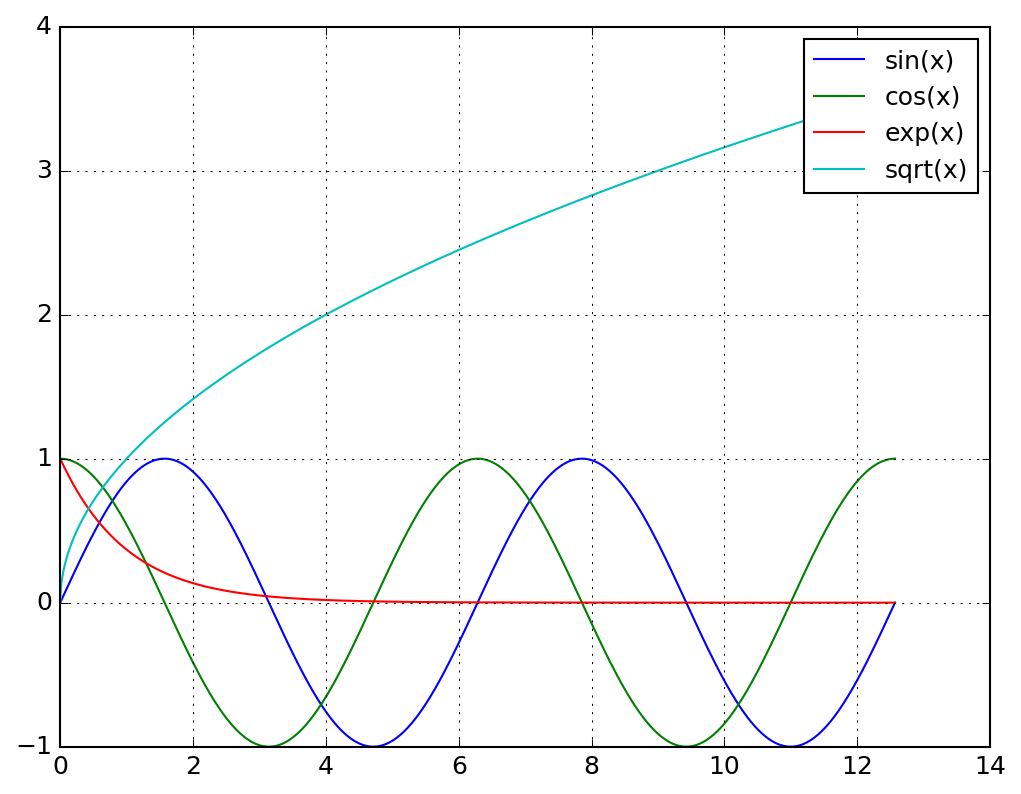
データを可視化するために、 matplotlib を使って、データをプロットしてみます。

example-17

import numpy as np
import matplotlib.pyplot as plt

fig, ax = plt.subplots()
x = np.linspace(0, 4 * np.pi, 1000)
ax.plot(x, np.sin(x), label="sin(x)")
ax.plot(x, np.cos(x), label="cos(x)")
ax.plot(x, np.exp(-x), label="exp(x)")
ax.plot(x, np.sqrt(x), label="sqrt(x)")
ax.legend()
fig.savefig("plot.png")
plt.show()

プログラムを実行すると次のような図が得られます。

注意点としてobject型の場合、numpyの数学関数に渡すためにastype()でfloat 型に変換せねばなりません。以下の例をみてください。np.sqrt()にobjectを 渡すとエラーになります。

example-18

import numpy as np

CH4 = """
H  2.00000000 0.00000000 0.00000000 
H  3.25515949 1.25515949 0.00000000 
H  3.25515949 0.00000000 1.25515949 
H  2.00000000 1.25515949 1.25515949 
C  2.62757974 0.62757974 0.62757974
"""

data = np.array(CH4.split(), dtype=object).reshape((-1, 4))
data[:, 1:4] = data[:, 1:4].astype(float)

# H-C...のvector生成
vec = data[0:4, 1:4] - data[4, 1:4]  # object typeの演算は可能
print(vec.dtype) # object
# normの計算
vec2 = vec[:, 0]**2 + vec[:, 1]**2 + vec[:, 2]**2
# np.sqrtにobjectを渡すとエラー
# vec_norm = np.sqrt(vec2)
# astype(float)でfloatに変換 (深いコピー)
vec_norm = np.sqrt(vec2.astype(float))
# C-H距離のリスト
print(vec_norm)

統計関数、ソートと検索

合計や平均の計算等、統計関数の一部と、配列のソートと検索を行う関数を紹 介します。リスト変数で使えるsorted()関数やindex()メソッドよりも高速かつ柔軟な関 数がnumpyに準備されています。多次元の配列の場合、軸を選択した処理を行 うことができます。

統計処理を行う関数のマニュアルは、以下のURLにリストされていますが、い くつか代表的なものをピックアップして紹介します。

https://docs.scipy.org/doc/numpy-1.13.0/reference/routines.statistics.html

統計関数

関数	機能
sum(a[, axis])	軸にそった足し算を行う。
mean(a[, axis])	軸にそった平均値を返す
std(a[, axis])	軸にそった標準偏差を返す
histogram(a, bins=n or ())	ヒストグラムを生成します。binsが整数ならデータ範囲を等しくn分割 した区分とします。binsにリストを渡せば区分のエッジを指定するこ とになります。

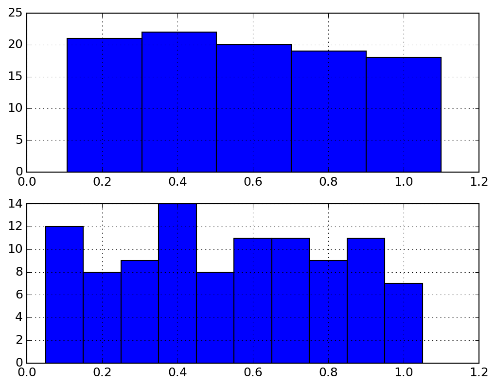
統計関数を使う計算例を示します。ヒストグラムは、乱数で適当な数字を生成 してプロットしています。

example-19

import numpy as np
import matplotlib.pyplot as plt

x = np.linspace(1, 12, 12, dtype=int)
print(x)  # [ 1  2  3  4  5  6  7  8  9 10 11 12]

# ベクトルの平均値と標準偏差の計算 
print(np.mean(x)) # 6.5  (重み付き平均するならnp.average())
print(np.std(x))  # 3.45205252953

x = x.reshape((3, 4))
print(x)  # [[ 1  2  3  4] 
          #  [ 5  6  7  8] 
          #  [ 9 10 11 12]]
          
print(np.mean(x, axis=0))  # [ 5.  6.  7.  8.]
print(np.mean(x, axis=1))  # [  2.5   6.5  10.5]

# ヒストグラム
x = np.random.seed(777)
x = np.random.random(100)
# 区分の数を指定していしてヒストグラムを生成
hist, bin_edge = np.histogram(x, bins=5) 
print(bin_edge)  # [ 0.00738845  0.20582267  0.40425689  0.60269111  0.80112532  0.99955954]
print(bin_edge.size) # 6
print(hist)          # [21 22 20 19 18]
print(hist.size)     # 5
width = bin_edge[1:] - bin_edge[:-1]
v = bin_edge[:-1] + 0.5*width
fig, ax = plt.subplots(2)
ax[0].bar(v, hist, width)

# 区分のエッジを指定していしてヒストグラムを生成
bins = np.arange(0, 1.1, 0.1)  # [ 0.   0.1  0.2  0.3  0.4  0.5  0.6  0.7  0.8  0.9  1. ]
hist, bin_edge = np.histogram(x, bins=bins) # 区分の数を指定
width = bin_edge[1:] - bin_edge[:-1]
v = bin_edge[:-1] + 0.5*width
ax[1].bar(v, hist, width)
fig.savefig("histogram.png")
plt.show()

ヒストグラムのプロットで得られる結果は以下のとおりです。

ソートや検索を行う処理のマニュアルは、以下のURLになります。いくつか代 表的なものをピックアップして紹介します。

https://docs.scipy.org/doc/numpy-1.13.0/reference/routines.sort.html

ソート、検索、カウント関数

関数	機能
sort(a[, axis])	軸にそってsortした結果を返す
argsort(a[, axis])	軸にそってsortした要素番号の結果を返す
max(a[, axis])	軸にそった最大値の要素を返す
argmax(a[, axis])	軸にそった最大値の要素番号を返す
min(a[, axis])	軸にそった最小値の要素を返す
argmin(a[, axis])	軸にそった最小値の要素番号を返す

ソートと検索を行う例を示します。

example-20

import numpy as np

np.random.seed(7)
a = np.floor(np.random.random((3, 4))*100).astype(int)
print(a)  # [[ 7 77 43 72] 
          #  [97 53 50  7] 
          #  [26 49 67 80]]

print(np.sort(a, axis=0))  # [[ 7 49 43  7] 
                           #  [26 53 50 72] 
                           #  [97 77 67 80]]
                           
print(np.sort(a, axis=1))  # [[ 7 43 72 77] 
                           #  [ 7 50 53 97] 
                           #  [26 49 67 80]]

print(np.argsort(a, axis=0))  # [[0 2 0 1] 
                              #  [2 1 1 0] 
                              #  [1 0 2 2]]

print(np.argsort(a, axis=1))  # [[0 2 3 1] 
                              #  [3 2 1 0] 
                              #  [0 1 2 3]]

print(np.max(a))  # 97

print(np.max(a, axis=1))  # [77 97 80]

print(np.argmax(a))  # 4 (reshape(-1))された要素番号
print(np.argmax(a, axis=0))  # [1 0 2 2]

条件を満たす要素の数をカウントしたい場合、True/Falseの配列のsumを求め ればカウントできます(True:1, False:0)。

example-21

import numpy as np

np.random.seed(7)
a = (np.random.random((3, 4))*100).astype(int)
print(a)  # [[ 7 77 43 72] 
          #  [97 53 50  7] 
          #  [26 49 67 80]]

print(np.sum(50 < a))  # 6
print(np.sum((50 <= a) & (a < 70)))  # 3

線形代数計算

線形代数で学んだ行列の計算を行う関数をピックアップして紹介します。ここ では、numpyの配列を行列と読み替えて考えてください。

https://docs.scipy.org/doc/numpy-1.13.0/reference/routines.linalg.html

関数	機能
np.dot(a, b)	行列aと行列bの行列積の計算 @で代用可能
np.linalg.det(a)	行列式の計算
np.linalg.inv(a)	行列aの逆行列の計算
np.transpose(a)	行列aの転置の計算 .Tでも同じ
np.identify(n)	n次の単位行列を生成する。
np.linalg.eig(a)	aの固有値と固有ベクトルを返す。固有値(w)と、固有値に対応した固有ベクトル(v)(長さで規格化されている)
np.linalg.solve(a, b)	係数行列aとベクトルbを渡すとxを返す。 ax = b

行列積の計算は、行列の形に気をつけてください。A(m,n)*B(n,l)=C(m,l)のよ うにサイズが代わります。ここで、Aの列(n)とBの行(n)が揃ってなければ計算 できません。

example-22

import numpy as np

# 行列積の計算 (m,n)*(n*l)=(m,l)のサイズになる
a = np.linspace(1, 4, 4, dtype=int)                    # 1x4の行列
b = np.linspace(1, 12, 12, dtype=int).reshape((4, 3))  # 4x3の行列
c = np.linspace(1, 12, 12, dtype=int).reshape((3, 4))  # 3x4の行列
print(a @ b)  # [70 80 90]
print(b @ c)  # [[ 38  44  50  56] 
              #  [ 83  98 113 128] 
              #  [128 152 176 200] 
              #  [173 206 239 272]]

np.random.seed(7)
a = np.floor(np.random.random((3, 4))*100).astype(int)
print(a)  # [[ 7 77 43 72] 
          #  [97 53 50  7] 
          #  [26 49 67 80]]

print(a.T)  # [[ 7 97 26] 
            #  [77 53 49] 
            #  [43 50 67] 
            #  [72  7 80]]

b = a[:, 0:3] # 正方行列をスライス
print(b)  # [[ 7 77 43] 
          #  [97 53 50] 
          #  [26 49 67]]

print(np.linalg.det(b))  # -247491.0
b_ = np.linalg.inv(b)

print(np.round(b_, 6))   # [[-0.004449  0.012332 -0.006348] 
                         #  [ 0.021007  0.002622 -0.015439] 
                         #  [-0.013637 -0.006703  0.02868 ]]

print(np.round(b_ @ b))  # [[ 1. -0. -0.] 
                         #  [ 0.  1.  0.] 
                         #  [-0. -0.  1.]]

print(np.round(b @ b_))  # [[ 1. -0.  0.] 
                         #  [-0.  1. -0.] 
                         #  [-0. -0.  1.]]
                         
w, v = np.linalg.eig(b)
print(w)  # [ 159.00801699  -58.57861335   26.57059636]
print(v)  # [[-0.49894052 -0.72331637 -0.27458389] 
          #  [-0.69850001  0.68072762 -0.52108324] 
          #  [-0.51298741 -0.11585912  0.80813114]]
print(w[0]*w[1]*w[2]) # -247491.0

具体的に数学の問題をいくつか解いてみます。np.solve()を使って以下の連 立方程式を解いてみます。

\[\begin{split} 3x + 2y + 8z = 3 \\ 2y = 9z \\ -10x + y + 4 = 9z\end{split}\]

まず連立一次方程式を行列で書き直します。

\[\begin{split}\begin{bmatrix} 3\\ 0\\ -4 \end{bmatrix} = \begin{bmatrix} 3 & 2 & 8\\ 0 & 2 & -9\\ -10 & 1 & -9\\ \end{bmatrix} \begin{bmatrix} x\\ y\\ z \end{bmatrix}\end{split}\]

3つの連立一次方程式程度の計算は、一瞬でといてくれます。

example-23

import numpy as np

A = np.array([[3, 2, 8],
              [0, 2, -9],
              [-10, 1, -9]], dtype=float)
b = np.array([3, 0, -4], dtype=float)
x = np.linalg.solve(A, b) # [ 0.34824281  0.51757188  0.11501597]

# 計算結果を確かめる
print(np.round(A @ x, 3))   # [ 3.  0. -4.]
print(np.linalg.inv(A) @ b) # [ 0.34824281  0.51757188  0.11501597]

回転行列を使って分子を回転させる操作を行ってみましょう。細かい回転行列 はwikipediaでも参照してください。線形代数でもでてきたかと思います。任 意の座標を軸回りに \(\theta\) 回転させることができます。

https://ja.wikipedia.org/wiki/%E5%9B%9E%E8%BB%A2%E8%A1%8C%E5%88%97

3次元の場合、 \(x, y, z\) の回転行列 \(Rx, Ry, Rz\) は以下のとおりです。

\[\begin{split}Rx(\theta) = \begin{bmatrix} 1 & 0 & 0\\ 0 & \cos\theta & -\sin\theta\\ 0 & \sin\theta & \cos\theta\\ \end{bmatrix} \quad Ry(\theta) = \begin{bmatrix} \cos\theta & 0 & \sin\theta\\ 0 & 1 & 0\\ -\sin\theta & 0 & \cos\theta\\ \end{bmatrix} \quad Rz(\theta) = \begin{bmatrix} \cos\theta & -\sin\theta & 0\\ \sin\theta & \cos\theta & 0\\ 0 & 0 & 1\\ \end{bmatrix} \quad\end{split}\]

もとの座標 \((x, y, z)\) を \(\theta\) だけ回転させた座標 \((x', y' ,z')\) は、次のように計算できます(\(x\) 軸回りに回転させる場合)。

\[\begin{split}\begin{bmatrix} x'\\ y'\\ z'\\ \end{bmatrix} = \begin{bmatrix} 1 & 0 & 0\\ 0 & \cos\theta & -\sin\theta\\ 0 & \sin\theta & \cos\theta\\ \end{bmatrix} \begin{bmatrix} x\\ y\\ z\\ \end{bmatrix}\end{split}\]

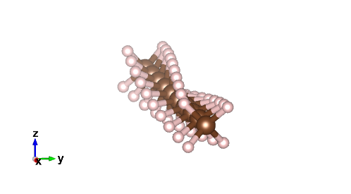
CH4をx方向に10度ずつ回しながらx方向に2Ang.シフトさせたxyzファイルを10個 生成してみます。

example-24

import numpy as np

CH4 = """
H  2.00000000 0.00000000 0.00000000 
H  3.25515949 1.25515949 0.00000000 
H  3.25515949 0.00000000 1.25515949 
H  2.00000000 1.25515949 1.25515949 
C  2.62757974 0.62757974 0.62757974
"""

def CalcData(CH4, theta, shift):
    """
    CH4: ベースのCH4データ
    theta: ベースのCH4をx軸回りに回転させる角度 (deg.)
    shift: ベースのCH4をx軸回方向にシフトさせる量
    """
    theta = theta * np.pi/180
    Rx = np.array([[1, 0, 0],
                   [0, np.cos(theta), -np.sin(theta)],
                   [0, np.sin(theta), np.cos(theta)]])
    CH4_new = np.copy(CH4)
    # r.T=(A @ r).T -> r.T @ A.T
    CH4_new[:, 1:4] = CH4[:, 1:4].astype(float) @ Rx.T
    CH4_new[:, 1] = CH4_new[:, 1] + shift
    return CH4_new

base = np.array(CH4.split(), dtype=object).reshape((5, 4))
base[:, 1:4] = base[:, 1:4].astype(float)
# Cを原点にする
base[:, 1:4] = base[:, 1:4] - base[base[:, 0] == "C", 1:4]

# データを保存する配列を準備(0行4列)
data = np.empty((0, 4))
# 原点のCH4を追加
for i in range(10):
    d = CalcData(base, i*10, i*2)
    data = np.concatenate((data, d), axis=0)

# xyzファイルの出力
outfile = "CH4-rotate.xyz"
o = open(outfile, "w")
o.write("{}\n".format(len(data)))
o.write("CH4 rotate and shift\n")
for d in data:
    o.write("{} ".format(d[0]))
    o.write("{} ".format(d[1]))
    o.write("{} ".format(d[2]))
    o.write("{} ".format(d[3]))
    o.write("\n")
print(outfile, "was created.")

プログラムを実行すると CH4-rotate.xyz が生成されます。作成したxyzファイルをvestaで開いた結果を下にしめします。x軸に沿ってぐるぐる回っていることがわかるかと思います。

多項式近似、内挿

実験データを下式のような多項式でフィッテングすることはよくあります。こ こで、 \(n\) はdegree(次数)で自分でモデルを決めてフィッテングしま す。np.polyfit()を使えば、簡単に多項式フィットを行うことができます。

https://docs.scipy.org/doc/numpy-1.13.0/reference/generated/numpy.polyfit.html

\[f(x) = a_0 + a_1x + a_2x^2 + \cdots + a_nx^n = \sum_{i=0}^n a_i x^i\]

適当な多項式の関数にノイズを加えたデータを作成し、多項式でフィッテング してみます。xとyがデータ、degを次数として、np.polyfit(x, y, degree)を 呼び出せば \(a_i\) を戻り値として求めてくれます。np.polyfit()の戻 り値とxfをnp.polyvalに渡せば、多項式フィットしたyfを得ることができます。

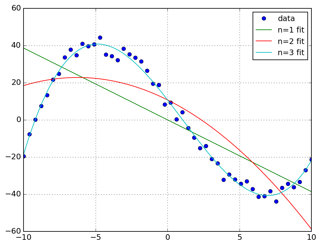
以下の多項式でテストデータを作成し、np.random.random()でノイズを印加し て、1, 2, 3次でフィッテングしたプログラムを例に示します。

\[\begin{split}&y = 0.1x^3 - 0.3x^2 - 10x + 5\\ &(a_3, a_2, a_1, a_0) = (0.1, -0.3, 10, 5)\end{split}\]

example-25

import numpy as np
import matplotlib.pyplot as plt

x = np.linspace(-10, 10, 50)
y = 0.1*x**3 - 0.3*x**2 - 10*x + 5
np.random.seed(0)
y = y + np.random.random(x.size) * 10  # ノイズの印加

op1 = np.polyfit(x, y, 1)  # n=1でフィット y = a1x + a0
op2 = np.polyfit(x, y, 2)  # n=2でフィット y = a2x**2 + a1x + a0
op3 = np.polyfit(x, y, 3)  # n=3でフィット y = a3x**3 + a2x**2 + a1x + a0

print(op1)
# [-3.8623472  -0.02851208]
print(op2)
# [ -0.30923446  -3.8623472   10.70003027]
print(op3)
# [  0.09852041  -0.30923446 -10.01156373  10.70003027]

xf = np.linspace(-10, 10, 1000)  # 多項式関数用のx
y1 = np.polyval(op1, xf)         # n=1でfitした結果
y2 = np.polyval(op2, xf)         # n=2でfitした結果
y3 = np.polyval(op3, xf)         # n=3でfitした結果

fig, ax = plt.subplots()
ax.plot(x, y, "o", label="data")
ax.plot(xf, y1, "-", label="n=1 fit")
ax.plot(xf, y2, "-", label="n=2 fit")
ax.plot(xf, y3, "-", label="n=3 fit")
ax.legend()
fig.savefig("polynominal.png")
plt.show()

3次の多項式フィットで求めた結果は以下のとおりになります。ノイズを印加しているので、元の関数の係数を完全に再現できていませんが近い結果を得ています。

\[(a_3, a_2, a_1, a_0) = (0.09852041, -0.30923446, -10.01156373, 10.70003027)\]

結果をプロットした図は以下のとおりです。

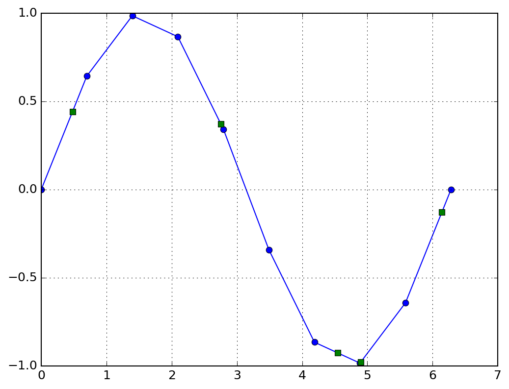
データの内挿は、np.interp()で行うことができます。内挿したいxの配列、デー タ点の配列(xp, yp)でnp.interp(x, xp, yp)に渡せば内挿したyデータが得ら れます。

https://docs.scipy.org/doc/numpy-1.13.0/reference/generated/numpy.interp.html

example-26

import numpy as np
import matplotlib.pyplot as plt

x = np.linspace(0, 2*np.pi, 10)
y = np.sin(x)

np.random.seed(7)
xi = np.random.random(5) * 2*np.pi  # 内挿するxデータ
yi = np.interp(xi, x, y)            # interp()でxの内挿取得

fig, ax = plt.subplots()
ax.plot(x, y, "o-")  # 実験データ
ax.plot(xi, yi, "s")     # 内挿データ
fig.savefig("interpolate.png")
plt.show()

結果をプロットした図は以下のとおりです。

クイズ

Q1

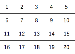
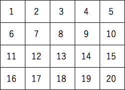
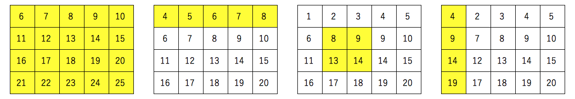
linspace()とreshape()を使って以下の配列を作成する。

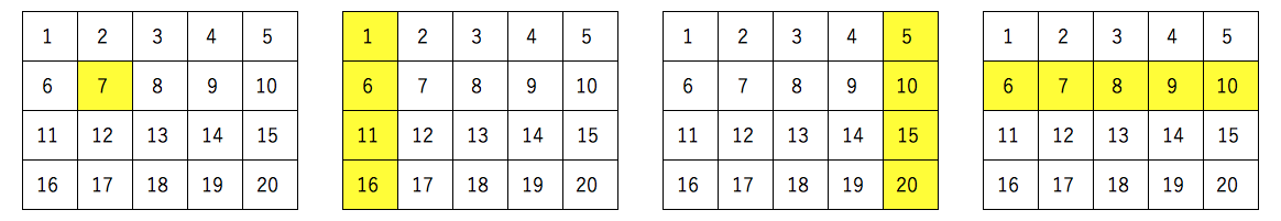
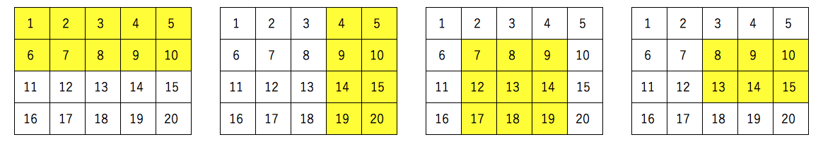
作成した配列のindexingにより黄色の配列を表示する。

import numpy as np

x = np.linspace(1, 20, 20).reshape(4, 5).astype(int)
print(x[1, 1])
print(x[:, 0].reshape(-1, 1))
print(x[:, -1].reshape(-1, 1))
print(x[1, :])
print(x[0:2, :])
print(x[:, 3:5])
print(x[1:4:, 1:4])
print(x[1:3:, 2:5])

Q2

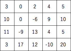
次の配列を直接入力して作成する。

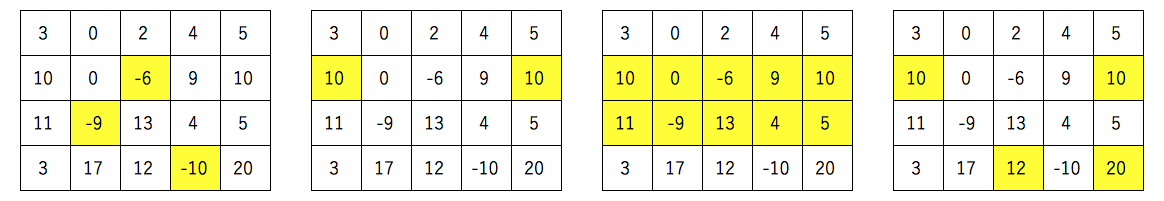
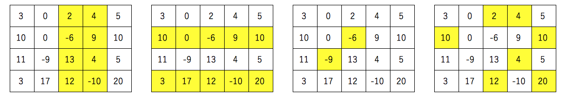
作成した配列からTrue, False(boolean)を使って(深いコピー)次の配列を表示する。 (注意)何通りもやり方があります。

import numpy as np

x = np.array([[3, 0, 2, 4, 5],
              [10, 0, -6, 9, 10],
              [11, -9, 13, 4, 5],
              [3, 17, 12, -10, 20]])

print(x[x < 0])
print(x[x == 10])
print(x[(x[:, 0] == 10) | (x[:, 0] == 11), :])
print(x[(x == 10) | (x == 12) | (x == 20)])
print(x[:, (x[0, :] == 2) | (x[0, :] == 4)])
print(x[(x[:, 4] == 10) | (x[:, 4] == 20), :])
print(x[(x < 0 ) & (x % 3 == 0)])
print(x[(x % 2 == 0) & (x != 0)])

Q3

linspace()とreshape()を使って以下の配列を作成する。

作成した配列から、indexing、深いコピーによるスライスとbroadcastingを組 み合わせて黄色のデータを表示させる。1文でデータを表示させること(注意)何通りもやり方が あります。

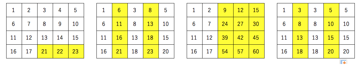
import numpy as np

x = np.linspace(1, 20, 20).reshape(4, 5).astype(int)
print(x + 5)
print(x[0, :] + 3)
print(x[1:3, 1:3] + 1)
print((x[:, 0] + 3).reshape(-1, 1))
print(x[3, 2:5] + 3)
print(x[:, [1, 3]] + 4)
print(x[:, 2:5]*3)
print(x[:, [1, 3]] + 1)

Q4

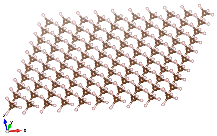
xy平面に2Ang.離してCH4を10x10個しきつめたxyzファイルを生成するプログラ ムを作成する。以下のforループの中の「自分で考える」のところにプログラ ムを書き加えて完成させる。

import numpy as np

CH4 = """
H  2.00000000 0.00000000 0.00000000
H  3.25515949 1.25515949 0.00000000
H  3.25515949 0.00000000 1.25515949
H  2.00000000 1.25515949 1.25515949
C  2.62757974 0.62757974 0.62757974
"""

# Cを原点にする
base = np.array(CH4.split(), dtype=object).reshape((5, 4))
base[:, 1:4] = base[:, 1:4].astype(float)
base[:, 1:4] = base[:, 1:4] - base[base[:, 0] == "C", 1:4]

data = np.empty((0, 4))
for i in range(10):
    for j in range(10):
       """自分で考える"""

# xyzファイルの出力
outfile = "CH4-problem.xyz"
o = open(outfile, "w")
o.write("{}\n".format(len(data)))
o.write("CH4 rotate and shift\n")
for d in data:
    o.write("{} ".format(d[0]))
    o.write("{} ".format(d[1]))
    o.write("{} ".format(d[2]))
    o.write("{} ".format(d[3]))
    o.write("\n")
print(outfile, "was created.")

生成するxyzファイルは下図のような構造です。

CH4-problem.xyz

import numpy as np

CH4 = """
H  2.00000000 0.00000000 0.00000000 
H  3.25515949 1.25515949 0.00000000 
H  3.25515949 0.00000000 1.25515949 
H  2.00000000 1.25515949 1.25515949 
C  2.62757974 0.62757974 0.62757974
"""

# Cを原点にする
base = np.array(CH4.split(), dtype=object).reshape((5, 4))
base[:, 1:4] = base[:, 1:4].astype(float)
base[:, 1:4] = base[:, 1:4] - base[base[:, 0] == "C", 1:4]

data = np.empty((0, 4))
for i in range(10):
    for j in range(10):
        data_ = np.copy(base)
        data_[:, 1] = data_[:, 1] + j*2
        data_[:, 2] = data_[:, 2] + i*2
        data = np.concatenate((data, data_), axis=0)

# xyzファイルの出力
outfile = "CH4-problem.xyz"
o = open(outfile, "w")
o.write("{}\n".format(len(data)))
o.write("CH4 rotate and shift\n")
for d in data:
    o.write("{} ".format(d[0]))
    o.write("{} ".format(d[1]))
    o.write("{} ".format(d[2]))
    o.write("{} ".format(d[3]))
    o.write("\n")
print(outfile, "was created.")

Q5

以下の連立方程式をnp.solve()を使って解いて \(a_0, a_1, a_2, a_3\) を求める。

\[\begin{split}3a_0 + 8.2a_1 = -2a_3\\ 2.3a_2 + 9.3a_3 = 0\\ -2.3a_0 + 1.8a_1 + 8a_2 + 7.2a_3 = 13\\ 0.8a_0 + 7.3a_1 = 5.3a_2 + 9a_3\end{split}\]

import numpy as np

A = [[3, 8.2, 2, 0],
     [0, 0, 2.3, 9.3],
     [-2.3, 1.8, 8, 7.2],
     [0.8, 7.3, 5.3, -9]]
b = [0, 0, 13, 0]

x = np.linalg.solve(A, b)
# 確認
print(x)
print(np.round(A @ x.T, 3))

Q6

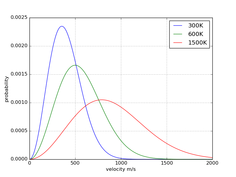
300K, 600K, 1500KでのArの速度分布をマクスウェル速度分布の式に従ってプ ロットする。以下のプログラムのHOGE部分を自分で考えてプログラムを完成さ せる。プロットすると下図のようなグラフが得られます。

\[\begin{split}&f(v) = 4\pi v^2\left(\frac{m}{2\pi R T}\right)^{3/2} \exp\left(-\frac{mv^2}{2RT}\right)\\ &m: {\rm Ar}質量\ {\rm kg/mol}\\ &R: ガス定数\quad 8.3144621\ {\rm J/K/mol}\\ &T: 温度\ {\rm K}\end{split}\]

import numpy as np
import matplotlib.pyplot as plt

R = 8.3144621       # J/K/mol
m = 39.948*1e-3     # kg/mol

fig, ax = plt.subplots()
v = np.linspace(0, 2000, 1000)  # m/s
A = 4*np.pi*v**2

f = HOGE
g = HOGE
h = HOGE

ax.plot(v, f, label="300K")
ax.plot(v, g, label="600K")
ax.plot(v, h, label="1500K")
ax.legend()
ax.set_xlabel("velocity m/s")
ax.set_ylabel("probability")
fig.savefig("problem-05.png")
plt.show()

作成したプログラムを改造して以下の計算を行う。

• 速度分布が規格化(積分すると1)されていることを確認する。300Kで得た分布の各点を長方形として、全領域の足し算で良いです。

• 300K, 600K, 1500Kでもっとも頻度の高い速度

• 300K, 600K, 1500Kの平均速度

• 300K, 600K, 1500Kで1000 m/s以上のArの割合(%)

すべて数式として解析的に得ることができますが、プログラムを使ってデータから計算すること。

import numpy as np
import matplotlib.pyplot as plt

R = 8.3144621       # J/K/mol
m = 39.948*1e-3     # kg/mol

v = np.linspace(0, 2000, 1000)  # m/s
A = 4*np.pi*v**2

f = A*(m/(2*np.pi*R*300))**(1.5)*np.exp(-m*v**2/(2*R*300))
g = A*(m/(2*np.pi*R*600))**(1.5)*np.exp(-m*v**2/(2*R*600))
h = A*(m/(2*np.pi*R*1500))**(1.5)*np.exp(-m*v**2/(2*R*1500))

# 速度分布が規格化(積分すると1)されていることを確認する
width = v[1] - v[0]
print("300K area: {:.2f}".format(np.sum(f * width)))
print("600K area: {:.2f}".format(np.sum(g * width)))
print("1500K area: {:.2f}".format(np.sum(h * width)))

# 300K, 600K, 1500Kでもっとも確率頻度の高い速度
print("300K maximum v: {:.2f}".format(v[np.argmax(f)]))
print("600K maximum v: {:.2f}".format(v[np.argmax(g)]))
print("1500K maximum v: {:.2f}".format(v[np.argmax(h)]))

# 300K, 600K, 1500Kの平均速度。
print("300K area: {:.2f}".format(np.sum(f * v * width)))
print("600K area: {:.2f}".format(np.sum(g * v * width)))
print("1500K area: {:.2f}".format(np.sum(h * v * width)))

# 300K, 600K, 1500Kで1000 m/s以上のArの割合(%)
idx = v > 1000
s = "more than 1000 m/s at {}: {:.2f}"
print(s.format(300, np.sum(f[idx] * width * 100)))
print(s.format(600, np.sum(g[idx] * width * 100)))
print(s.format(1500, np.sum(h[idx] * width * 100)))

# plotting
fig, ax = plt.subplots()
ax.plot(v, f, label="300K")
ax.plot(v, g, label="600K")
ax.plot(v, h, label="1500K")
ax.grid()
ax.legend()
ax.set_xlabel("velocity m/s")
ax.set_ylabel("probability")
fig.savefig("problem-05.png")
plt.show()

Q7

以下の図のような1辺が100 Ang.の立方体にArが10000個入った Ar.xyz がある。 立方体の中心座標は、(x, y, z) = (0, 0, 0)になっている。

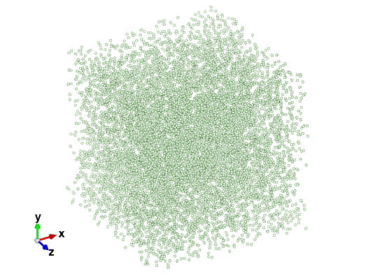
• x座標が-2から2の範囲に存在するArを抜き出してxyzファイルを作成する。

• 立方体の中心から40 Ang.以内に存在するArを抜き出してxyzファイルを作成する。

それぞれ以下のようなxyzファイルが得られます。

import numpy as np

# LxLxLに10000個の原子を少なくとも2Ang.離してランダム置く
L = 100
data = np.array([[0, 0, 0]])
while len(data) < 10000:
    p = np.random.random(3) * L - 0.5*L
    r = np.sum((p - data)**2, axis=1)
    if np.all(r > 2):
        data = np.concatenate((data, [p]), axis=0)

o = open("Ar.xyz", "w")
o.write("{}\n".format(len(data)))
o.write("\n")
for d in data:
    o.write("Ar {} {} {}\n".format(d[0], d[1], d[2]))

# -2<x<2の面
t = 2
idx = (-t < data[:, 0]) & (data[:, 0] < t)
data_ = data[idx, :]
o = open("Ar_layer.xyz", "w")
o.write("{}\n".format(len(data_)))
o.write("\n")
for d in data_:
    o.write("Ar {} {} {}\n".format(d[0], d[1], d[2]))

# r=40のball 
r = np.sqrt(np.sum(data**2, axis=1))
data_ = data[r < 40, :]
o = open("Ar_ball.xyz", "w")
o.write("{}\n".format(len(data_)))
o.write("\n")
for d in data_:
    o.write("Ar {} {} {}\n".format(d[0], d[1], d[2]))

Q8

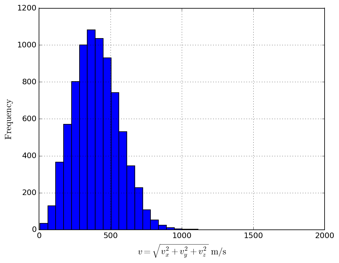
温度300Kの容器に存在するArガスの速度ベクトル(8000個のAr分)のデータ Ar_velocity.dat を読んで、np.histogram()により速度のヒストグラムを作成しプロットする。問題5と同じ分布関数になりますが、区分の幅(bins)で高さが変わります。速度範囲を20分割してヒストグラムを作成しプロットした結果を下に示します。

import numpy as np
import matplotlib.pyplot as plt

lines = open("Ar/Ar.lammpstrj").readlines()[9:]
data = np.array(" ".join(lines).split(), dtype=float).reshape((-1, 3))
data = data * 1e-10/1e-15 # m/s
o = open("Ar_velocity.dat", "w")
o.write("# {:15s}  {:16s} {:16s}\n".format("vx(m/s)", "vy(m/s", "vz(m/s)"))
for d in data:
    o.write("{:16.8e} {:16.8e} {:16.8e}\n".format(d[0], d[1], d[2]))
print("Ar_velocity.dat was created.")

v = np.sqrt(np.sum(data**2, axis=1))
hist, bins = np.histogram(v, bins=20)
w = bins[1] - bins[0]
x = bins[0:-1] + 0.5*w
fig, ax = plt.subplots()
ax.bar(x, hist, width=1.0*w, align="center")
# ax.plot(x, hist)
ax.set_xlim(0, 2000)
ax.set_xlabel("$v = \sqrt{v_x^2 + v_y^2 + v_z^2}\ {\\rm m/s}$")
ax.set_ylabel("${\\rm Frequency}$")
fig.savefig("problem-07.png")
plt.show()

Q9

反応次数が1(一次反応)の化学反応の場合、反応物の濃度 \([A]\) は時間の経過とともに初期濃度 \([A]_0\) から以下の式に従って減少する。

\[\begin{split}&[A] = [A]_0\exp\left(-kt\right)\\ &k(T): 速度定数\ s^{-1}\\ &t: 時間\ s\\\end{split}\]

両辺の自然対数をとれば以下の一次の関係式が得られる。

\[\ln([A]) = \ln([A]_0) - kt\]

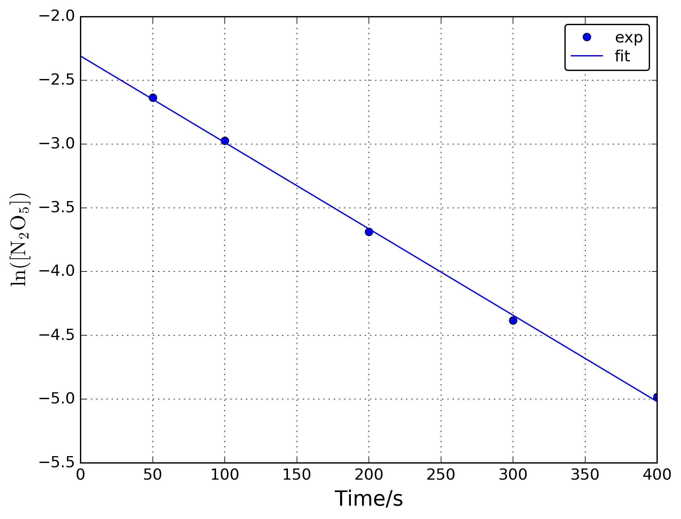
以下の反応について、時間と \({\rm [N_2O_5]}\) のデータを実験から得た。

得られたデータは以下のとおり。np.polyfit()を用いて直線フィットし反応速度 \(k\) と初期濃度 \({\rm [N_2O_5]_0}\) を求める。

Time/s      [N2O5]/M
50          0.0717
100         0.0511
200         0.0250
300         0.0125
400         0.00685

実験データから以下のような図を作成すれば、 \(k\) と \({\rm [N_2O_5]_0}\) が求まります。

import numpy as np
import matplotlib.pyplot as plt

data = """
Time/s      [N2O5]/M
50          0.0717
100         0.0511
200         0.0250
300         0.0125
400         0.00685"""

data = np.array(data.split()).reshape((-1, 2))
data = data[1:, :].astype(float)
x = data[:, 0]
y = np.log(data[:, 1])
o = np.polyfit(x, y, 1)
print("k: {} 1/s".format(-o[0]))
print("[N2O5]0: {} M".format(np.exp(o[1])))

xf = np.linspace(0, x[-1], 2)
yf = np.polyval(o, xf)
fig, ax = plt.subplots()
ax.plot(x, y, "bo", label="exp")
ax.plot(xf, yf, "b-", label="fit")
ax.set_xlabel("Time/s")
ax.set_ylabel("${\\rm \ln([N_2O_5])}$")
ax.legend()
fig.savefig("rate_const.png")
plt.show()