ランダムウォーク
一定の時間ステップ毎にランダムに方向を変えながら粒子が並進運動する現象 をランダムウォーク(酔歩)と呼びます。酔っ払った人がフラフラ歩いていてど こに向かっているかわからない動きにちなんで酔歩とも呼びます
自然科学の分野では微粒子のブラウン運動や株価の動きはランダムウォークに なることが知られています。
1粒子だけだと、ど こまで進むか(変位)を予測できませんが、多数の粒子(\(N\))のランダム ウォークを観測して平均自乗変位を求めると拡散係数(\(D\))と次の関係 が成立します。
ここで \(dim\) は次元数で2次元だと2、3次元だと3です。
注釈
拡散方程式から導かれる粒子分布(正規分布)から平均自乗変位を計算すれば、上式は導くことができます。
2次元のランダムウォークシミュレーション
ランダムウォークシミュレーションは、乱数を発生させて時間ステップ毎にラ ンダムな方向に多数の粒子を進めていけば実装できます。二次元でのランダム ウォークシミュレーションを行って、平均自乗変位と時間の関係から拡散係数 を求めてみます。1ステップで移動する距離は一定とし、移動方向 \(\theta\) を乱数を使ってランダムに決定して粒子を動かします。全粒 子の時間毎の変位を求めたら時間ごとの平均自乗変位(rms; root-mean-square) を求めて直線近似し、傾きから拡散係数を求めてみます。
プログラムはforを使わずにステップ数x粒子数の乱数を一度で発生させ、各時 間ステップ毎の方向を決めて、np.cumsum()で足し上げて各時間ステップでの 位置を計算しています。1ステップの距離や時間の単位は、自分で決める必要 があります。
#!/usr/bin/env python
import numpy as np
import matplotlib.pyplot as plt

# 図の体裁
plt.style.use('classic')
plt_dic = {}
plt_dic['legend.fancybox'] = True
plt_dic['legend.labelspacing'] = 0.3
plt_dic['legend.numpoints'] = 3
plt_dic['figure.figsize'] = [8, 6]
plt_dic['axes.grid'] = True
plt_dic['legend.fontsize'] = 12
plt_dic['axes.labelsize'] = 14
plt.rcParams.update(plt_dic)

# シミュレショーンのパラメータ
p_dic = {}
p_dic['step'] = 1000   # ステップ数
p_dic['atom'] = 500    # 粒子数
p_dic['r'] = 1         # 1ステップの距離
np.random.seed(3)      # いつも同じ乱数列を生成するため

# 粒子数xステップ数の乱数生成
rnd = np.random.random((p_dic['atom'], p_dic['step']))
# radianに変換
rnd = rnd * 2 * np.pi
# 全粒子のt=0は原点
x = np.zeros((p_dic['atom'], 1))
y = np.zeros((p_dic['atom'], 1))
# 各ステップでの移動座標を生成
x = np.concatenate((x, np.cos(rnd)), axis=1)
y = np.concatenate((y, np.sin(rnd)), axis=1)
# 時間で積算
x = np.cumsum(x, axis=1)
y = np.cumsum(y, axis=1)
# 平均自乗変位の計算
r = np.mean(x**2 + y**2, axis=0)

t = np.linspace(0, p_dic['step'], p_dic['step'] + 1)
# 後半のデータを使って、rms = 4Dtでfitting
bound = int(p_dic['step'] * 0.5)
t_fit, r_fit = t[bound:], r[bound:]
out = np.polyfit(t_fit, r_fit, 1)
r_cal = np.polyval(out, t_fit)
D = out[0]/4
print("Diffusion coefficient = {:.3g}".format(D))


# 図の作成
fig, ax = plt.subplots()
lim = np.max([x, y])
for i in range(6):  # 6粒子の軌跡をプロット
    ax.plot(x[i], y[i], label="{}".format(i+1))
ax.legend(loc="best")
ax.set_xlabel('x')
ax.set_ylabel('y')
# x,yのrangeを揃える
lim = np.max([np.abs(ax.get_xlim()), np.abs(ax.get_ylim())])
ax.set_xlim(-lim, lim)
ax.set_ylim(-lim, lim)
fig.savefig("randwalk.png")

fig, ax = plt.subplots()
ax.plot(t, r, ".", ms=2.0, label="data")
ax.plot(t_fit, r_cal, "-", label="fit")
ax.legend(loc="best")
ax.set_xlabel('step')
ax.set_ylabel('rms distance')
fig.savefig("rms-time.png")

plt.show()
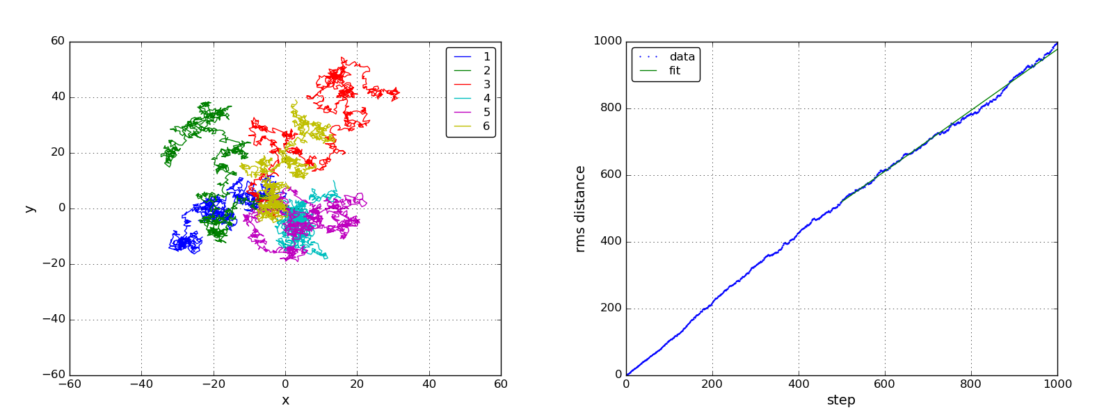
プログラムを実行すると拡散係数と次のような図が得られます。6粒子だけの 粒子の軌跡を描いています(左)。平均自乗変位の後ろ半分のデータを直線フィッ トして拡散係数を求めています(右)。
Diffusion coefficient = 0.229
クイズ
Q1
2次元のランダムウォークシミュレーションのプログラムを3次元のプログラム に変更する。
Q2
各時間ステップでの粒子の運動方向を \(0, \pi/2, -\pi/2, \pi\) の4 方向に限定してシミュレーションするよう変更する。